paper

目录

1. Attention Is All You Need : Transformer
2. End-to-End Object Detection with Transformers: DETR
3. AN IMAGE IS WORTH 16X16 WORDS: TRANSFORMERS FOR IMAGE RECOGNITION AT SCALE: Vision Transformer
4. Incremental-DETR: Incremental Few-Shot Object Detection via Self-Supervised Learning
5. Lightweight Transformer for Multi-Modal Object Detection (Student Abstract)
6. Self-supervised Label Augmentation via Input Transformations
7. Learn More for Food Recognition via Progressive Self-Distillation
8. Solving Math Word Problems concerning Systems of Equations with GPT-3
9. Curriculum Temperature for Knowledge Distillation
10. SHARPNESS-AWARE MINIMIZATION FOR EFFICIENTLYIMPROVING GENERALIZATION
11. Adaptive Hierarchy-Branch Fusion for Online Knowledge Distillation
12. Peeling the Onion: Hierarchical Reduction of Data Redundancy for Efficient Vision Transformer Training
13. Class Incremental Learning for Task-Oriented Dialogue System with Contrastive Distillation on Internal Representations (Student Abstract)
14. Improving Training and Inference of Face Recognition Models via Random Temperature Scaling
15. De-biased Teacher: Rethinking IoU Matching for Semi-supervised Object Detection
16. Grouped Knowledge Distillation for Deep Face Recognition

泛读文章

3. Can Bad Teaching Induce Forgetting? Unlearning in Deep Networks Using an Incompetent Teacher

本文角度清奇，利用知识蒸馏使得模型变弱，有意忘记某些知识。比如某些公司的授权到期，需要忘记相关知识，两种方法，其一是重新训练，其二就是本文（知识蒸馏）。

4. SKDBERT: Compressing BERT via Stochastic Knowledge Distillation

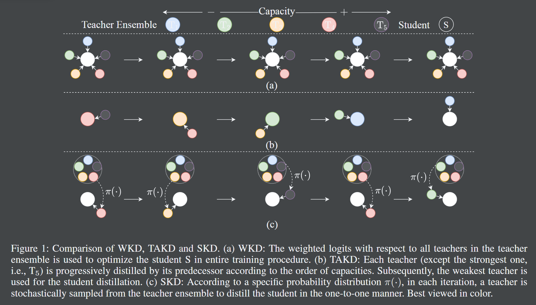
• 正如题目所言，本文采用了一种随机知识蒸馏的方法，具体来说，每次迭代中从很多老师中挑选一个老师，然后进行知识蒸馏。（老师们具有不同的容量层级）在能力基本没有损失的情况下，模型的大小减少了 40%。

本文提到了很多知识蒸馏的方法，可以参考。

5. Boosting Graph Neural Networks via Adaptive Knowledge Distillation

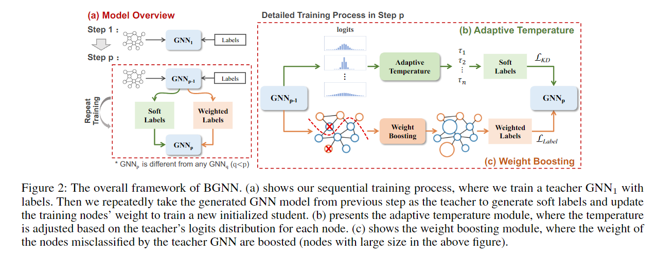
• 这篇论文是关于如何利用多个图神经网络（GNNs）的互补知识来提高一个学生GNN的性能。它提出了一个自适应的知识蒸馏（KD）框架，叫做BGNN，它可以顺序地将不同GNNs的知识转移到学生GNN中。它还引入了一个自适应温度模块和一个权重提升模块，来指导学生GNN有效地学习。这篇论文在节点分类和图分类任务上都取得了很好的效果，相比于原始的GNNs，分别提升了3.05%和6.35%。

作者认为，对于同一个GNN，采用不同的聚合方式，会学到不同的知识，现在希望互补的掌握这些知识，怎么办呢？采用知识蒸馏最好。 但这会有如下难点：

1. 传统的 KD teacher 要比 student 大，而本次任务中，两者相同容量
2. GNN 一般都比较浅

作者的创新在于，提出了这种构想，并引入了 自适应温度模块和权重提升模块

• 自适应温度模块，根据 teacher model 对于节点的 logits 分布，进行设计。具体依据是针对不同节点的梯度值。
• 权重提升模块，哪个节点对应的分类错误率高，就给哪个节点的权重提升。

正文

1. Attention Is All You Need : Transformer

先修知识

BLUE（Bilingual Evaluation Understudy）

机器翻译中的BLEU是一种用于评估机器翻译质量的指标，它通过计算机器翻译的句子和人工翻译的参考句子之间的n-gram匹配程度，来衡量机器翻译的精确度。n-gram是指连续的n个词，例如，unigram是一个词，bigram是两个词，trigram是三个词，依此类推。BLEU的取值范围是0到1，越接近1表示机器翻译越好，越接近0表示机器翻译越差。BLEU的计算公式如下：

其中，BP是简短惩罚因子，用于惩罚过短的机器翻译，防止机器翻译只输出少数几个词就获得高分。BP的计算公式如下：

其中，c是机器翻译的总长度，r是参考翻译的最佳匹配长度，即与机器翻译最接近的参考翻译的长度。

$p_n$是基于n-gram的改进精确度，用于计算机器翻译中的n-gram和参考翻译中的n-gram的匹配比例。$p_n$的计算公式如下：

$p*n = \frac{\sum*{\text{n-gram} \in C} \text{Count}_{\text{clip} }(\text{n-gram})}{\sum_{\text{n-gram} \in C} \text{Count}(\text{n-gram})}$

其中，C是机器翻译的句子，$\text{Count}(\text{n-gram})$是机器翻译中n-gram的出现次数，$\text{Count}_{\text{clip} }(\text{n-gram})$是机器翻译中n-gram的截断计数，即机器翻译中n-gram的出现次数与参考翻译中n-gram的最大出现次数的较小值。

$w_n$是n-gram的权重，一般取均匀权重，即$w_n = 1/N$，其中N是n-gram的最大阶数，通常取4。

简介

本文发表于 2017 年，提出了一种新的网络结构 Transformer，该结构完全基于 attention 机制，不再使用 CNN 和 RNN，因此可以并行计算，加快训练速度。Transformer 在机器翻译任务上取得了很好的效果，其后被广泛应用于其他任务中。

• 数据集：

  • WMT 2014 English-German： 包含了约 4.5 万对英德语句子，其中训练集包含 3.7 万对句子，开发集包含 0.5 万对句子，测试集包含 0.3 万对句子。句子来源于新闻、学术论文、书籍和网站等。

  • WMT 2014 English-French： 包含了约 35 万对英法语句子，其中训练集包含 29 万对句子，开发集包含 3 万对句子，测试集包含 3 万对句子。句子来源于新闻、学术论文、书籍和网站等。

• code

摘要

• 前人做的 sequence transduction 都是基于 RNN 或者 CNN
• 都用到了 encoder-decoder 结构
• 本文仍然基于 encoder-decoder 结构，但是不再使用 RNN 和 CNN，而是使用 attention 机制，这可以更好的并行。
• 所用指标为 BLUE，效果最好。

引言

• RNN 需要顺序的计算，无法并行。
• 已经有人使用了 attention 机制，但大都是和 RNN 或者 CNN 结合使用的。
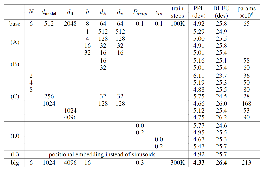
• 在 8 个 P100 上训练了 12 个小时。

背景

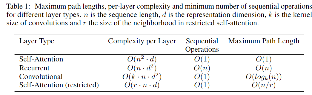
• 前人的方法还是没有解决长距离知识学习的问题，距离越长，所需要的计算越多。
• 在 Transformer 中，我们会通过 embedding 来固定维度，这会带来不好的影响，但所幸有 multi-head attention 来抵消。
• self-attention
• 前人已证，基于 recurrent attention mechanism 的效果更好，但还没有人仅用 attention 机制来做。

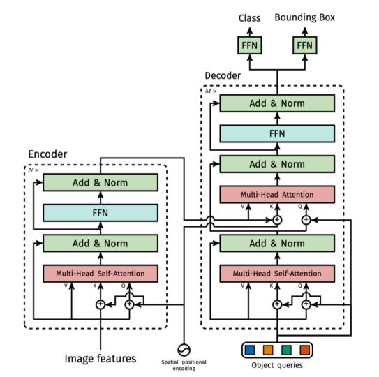
模型架构

• 沿用 Encoder-Decoder 结构，注意这里的 Decoder 是自回归的。（就是当前输入依赖于前面的输出）
• The Transformer - model architecture.

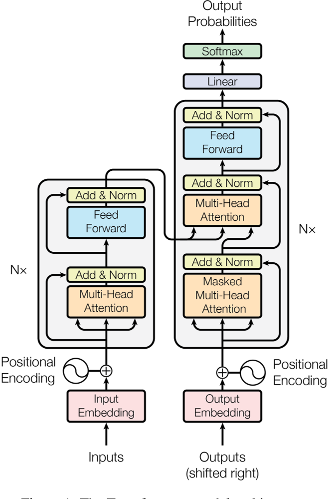
• Encoder

  • N = 6
  • 两层 sub-layer，分别是 multi-head self-attention 和 position-wise fully connected feed-forward network
  • 每层都有 residual connection，然后接 layer normalization
  • 为满足 residual connection，embedding 和 encoder 的输出维度都是 d_model = 512

• Decoder

  • N = 6
  • 三层 sub-layer，分别是 masked multi-head self-attention，multi-head self-attention 和 position-wise fully connected feed-forward network
  • 每层都有 residual connection，然后接 layer normalization
  • 对于编码器的输出执行多头注意力，K（键）和V（值）来自编码器的输出，而Q（查询）来自解码器的输出。这确保了解码器中的每个位置都可以访问编码器输出中的所有位置。
  • masked multi-head self-attention 用于防止解码器中的位置访问后续位置。这是通过将查询掩码为负无穷来实现的。

• Attention

  • Scaled Dot-Product Attention

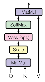
其中 queries 和 keys 的维度是 $d_k$，values 的维度是 $d_v$。 事实上， 这里是可以并行的，参见原文3.2.1

作者在这里指出，点积 要比 加性 效率高，具体谁更好，参见原文。

除以 $\sqrt{d_k}$ 是为了消除方差的影响，参见原文第四页页脚

• Multi-Head Attention

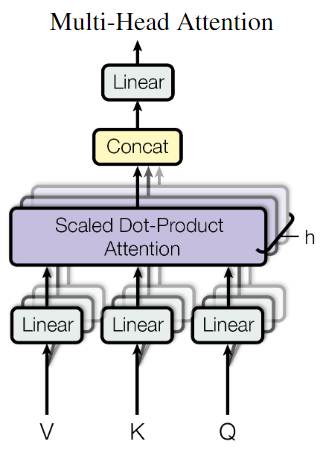
作者认为，直接将 queries，keys 和 values 映射到 $d_{model}$ 维度的空间中，可能会导致信息损失，因此，作者将 queries，keys 和 values 分别映射到 $d_k$，$d_k$ 和 $d_v$ 维度的空间中，然后进行 Scaled Dot-Product Attention，最后将多个结果拼接起来，再次映射到 $d_{model}$ 维度的空间中。

具体而言，文中设定 h = 8，即将 queries，keys 和 values 分别映射到 $d_k$ = $d_v$ = $d_{model}$/h = 64 维度的空间中，然后进行 Scaled Dot-Product Attention，最后将多个结果拼接起来，再次映射到 $d_{model}$ 维度的空间中。参见原文3.2.2

• Applications of Attention in our Model

  • quiries 来自前一个 decoder layer，keys 和 values 来自 encoder 的输出
  • encoder 包含 self-attention
  • 通过 mask 来防止 decoder 中的位置访问后续位置，具体而言，就是将 values 的后续位置 mask 为负无穷，这样过 softmax 之后，就会变成 0，即不会影响结果。

• Position-wise Feed-Forward Networks

$\mathcal{FFN} (x) = \mathbb{max} (0, x W_1 + b_1)W_2 + b_2$

其中输入和输出的维度都是 $d_{model}$ = 512，而中间层的维度是 $d_{ff}$ = 2048。

• embedding 作者将 input embedding 和 output embedding 共享参数，都是通过一个 线性层再加上一个softmax 来实现的。

在 embedding 的时候，所有的权重乘以 $\sqrt{d_{model} }$，这样可以使得 embedding 的结果的方差为 1，具体原因参考这篇帖子。

• Positional Encoding
  • attention 机制没有考虑到序列中词的位置信息。因此，作者在 embedding 后加入了位置编码，用于表示词的位置信息。
  • 维度为 $d_{model}$ = 512，位置编码的维度也是 512。便于求和

$\begin{aligned} \text{PE}_{(pos, 2i)} &= \sin(pos / 10000^{2i/d_{model} }) \\ \text{PE}_{(pos, 2i+1)} &= \cos(pos / 10000^{2i/d_{model} }) \end{aligned}$

其中，pos 是词在句子中的位置，i 是位置编码的维度。

Why Self-Attention?

• 可并行
• 距离远的词也可以相互影响
• 作者还提出了 局部注意力

Training

Results

其中大模型用 8 个 P100 GPU 训练了 3.5 天

Conclusion

• 本文提出了一种新的网络结构 Transformer，该结构完全基于 attention 机制，不再使用 CNN 和 RNN，因此可以并行计算，加快训练速度。
• Transformer 在机器翻译任务上取得了很好的效果，其后被广泛应用于其他任务中。
• 可以考虑 局部注意力
• 可以试试在 图像或音频 上应用 Transformer

2. End-to-End Object Detection with Transformers: DETR

先修知识

1. Hungarian algorithm : 匈牙利算法，用于解决指派问题

摘要

• 将目标检测视为 set prediction 问题，使用 Transformer 来解决。去除了 NMS、anchor、poposals 等。直接输出目标的位置和类别，真正的实现了端到端。
• 性能对标 Faster R-CNN，但速度更快。
• 数据集：COCO
• code

引言

• 现在都不是端对端，都是先生成一些 proposals，然后再分类，最后再回归。这样的结果受限于中间的这些操作。
• 虽然用到了 Transformer，但是却是并行出结果，不需要自回归。

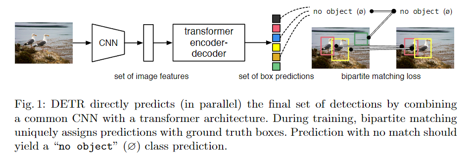
• 用到了 bipartite matching loss
• 在大物体上效果好，小物体上效果稍差
• 消融实验做的很好
• 很容易扩展到全景分割

相关工作

• 之前都是需要一些知识给模型，也就是先验知识，比如 anchor，NMS，proposals 等。
• 也有人通过 bipartite matching 来解决目标检测问题，但是是基于 RNN 的。

模型架构

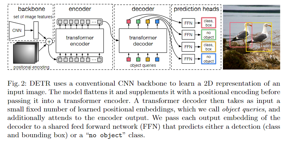
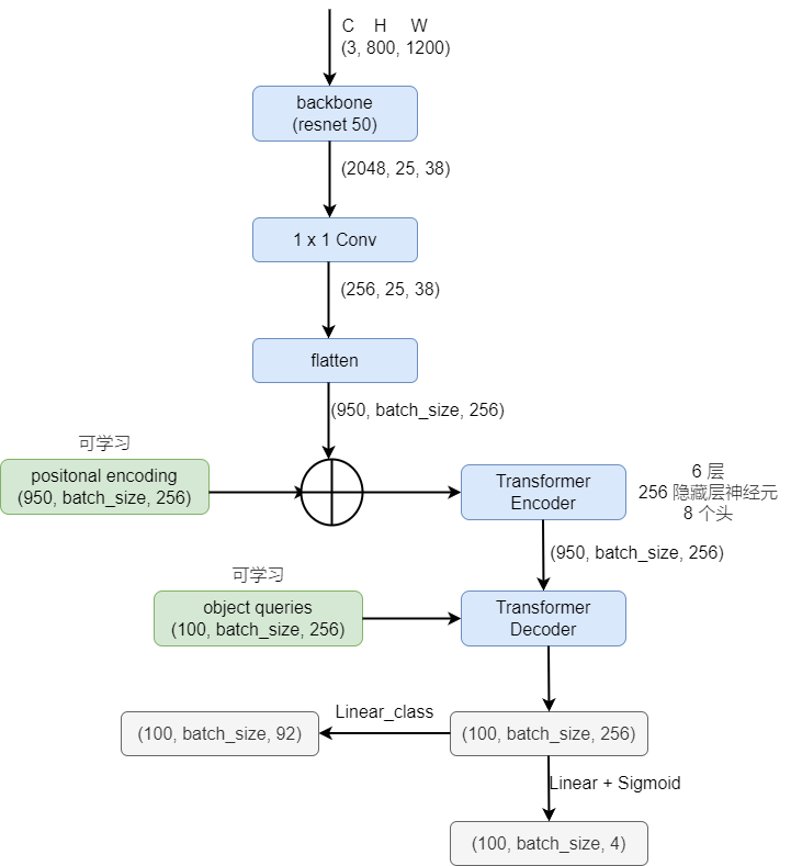
• object queries 是一个固定的向量，用于表示目标的个数，这里是 100 个（也就是 100 个框，根据数据集设定就好）。
• Matching cost 同时考虑了 class 和 box 的信息
• 仅对类别为 非空 的进行计算损失。
• 类别预测的损失，去除了 log，详见原文 3.1
• 边界框预测的损失，详见原文 3.1，使用了广义 IoU

loss 的计算分为如下几个部分：

首先通过 $\mathcal{L}_{match}$ 一对一的找到框，之后算损失：box loss + class loss

$\hat{\sigma} = \text{arg} \quad \text{min}_{\sigma \in \mathcal{\sigma}\_N} \sum_{i=1}^N \mathcal{L}_{\text{match} }(y_i, \hat{y}_{\sigma(i)})$

• $y_i = (c_i, b_i)$ 是 ground truth
• $c_i$ 是 class label，可以是 $\emptyset$
• $b_i$ 是 bounding box，(center x, center y, height, and width relative to the image size).
• $\hat{y}_i$ 是预测的结果，可以 padded with $\emptyset$ (no object) when N > the number of objects.
• $\hat{c_i}$ 是预测的类别
• $\hat{b_i}$ 是预测的 bounding box
• $\mathcal{\sigma(i)}$ is an index within a particular permutation of N elements.

$\mathcal{L}_{\text{match} }(y_i, \hat{y}_{\sigma(i)}) = - \mathbb{1}_{\{c_i \neq \emptyset\} } \hat{p}_{\sigma(i)}(c*i) + \mathbb{1}*{\{c*i = \emptyset\} } \mathcal{L}*{\text{box} }(b*i, \hat{b}*{\sigma(i)})$ - $\mathbb{1}_{\{c_i \neq \emptyset\} }$ 是指当 $c_i \neq \emptyset$ 时，取 1，否则取 0 - $\hat{p}_{\sigma(i)}(c_i)$ 是指预测的类别为 $c_i$ 的概率 - $\mathcal{L}_{\text{box} }(b_i, \hat{b}_{\sigma(i)})$ 是指预测的 bounding box 与 ground truth 的损失 $\mathcal{L}_{\text{box} }(b_i, \hat{b}_{\sigma(i)}) = \lambda*{iou} \mathcal{L}*{iou} (b*i, \hat{b}*{\sigma(i)}) + \lambda*{L_1} ||b_i - \hat{b}*{\sigma(i)}||\_1$

$L_1$ 损失较常用，但是对于小框和大框的损失处理有问题，因此作者加入了 $IoU$ 损失，详见原文

$\mathcal{L}_{\text{Hungarian} }(y, \hat{y}) = \sum_{i=1}^N [- \log \hat{p}_{\hat \sigma(i)}(c_i) + \mathbb{1}_{\{c_i \neq \emptyset\} } \mathcal{L}_{\text{box} }(b_i, \hat{b}_{\hat \sigma(i)})]$

事实上，作者还加了超参系数做平衡。这里使用了对数，而上文没有，是因为二者考虑的问题不一样，一个是考虑数值相对平衡，一个是考虑梯度相对平衡。

• positional encoding 也好，object queries 也好，都加入到了每一层 attention layer 的计算，
• 作者还加入了 Auxiliary decoding losses，也就是每一层的输出都会计算损失（但是所有的 FFN 共享参数），详见原文 3.2

实验

• 详细探究了每个组件的作用
• 全景分割的实验

结论

• 本文提出了一种新的目标检测方法 DETR，该方法使用 Transformer 来解决目标检测问题，去除了 NMS、anchor、poposals 等，直接输出目标的位置和类别，真正的实现了端到端。

附录代码

import torch
from torch import nn
from torchvision.models import resnet50

class DETR(nn.Module):

    def __init__(self, num_classes, hidden_dim, nheads, num_encoder_layer, num_decoder_layers):
        super().__init__()

        # Backbone: ResNet-50 without the last two layers (fully connected and pooling)
        self.backbone = nn.Sequential(*list(resnet50(pretrained=True).children())[:-2])

        # 1x1 Convolution to reduce channels from 2048 to hidden_dim
        self.conv = nn.Conv2d(2048, hidden_dim, 1)

        # Transformer layers
        self.transformer = nn.Transformer(hidden_dim, nheads, num_encoder_layer, num_decoder_layers)

        # Output layers
        self.linear_class = nn.Linear(hidden_dim, num_classes + 1)  # Class prediction (plus background)
        self.linear_bbox = nn.Linear(hidden_dim, 4)  # Bounding box prediction (4 coordinates)

        # Learnable positional embeddings
        self.query_pos = nn.Parameter(torch.rand(100, hidden_dim))  # Query positional embedding
        self.row_embed = nn.Parameter(torch.rand(50, hidden_dim // 2))  # Row positional embedding
        self.col_embed = nn.Parameter(torch.rand(50, hidden_dim // 2))  # Column positional embedding

    def forward(self, inputs):
        # Backbone feature extraction
        x = self.backbone(inputs)
        # 1x1 Convolution
        h = self.conv(x)

        # Get height (H) and width (W) of the feature map
        H, W = h.shape[-2:]

        # Positional embeddings
        pos = torch.cat([
            self.col_embed[:W].unsqueeze(0).repeat(H, 1, 1),
            self.row_embed[:H].unsqueeze(1).repeat(1, W, 1)
        ], dim=-1).flatten(0, 1).unsqueeze(1)

        # Flatten and permute for transformer input
        h = self.transformer(pos + h.flatten(2).permute(2, 0, 1), self.query_pos.unsqueeze(1))

        # Output predictions
        return self.linear_class(h), self.linear_bbox(h).sigmoid()

# Instantiate the model
detr = DETR(num_classes=91, hidden_dim=256, nheads=8, num_encoder_layer=6, num_decoder_layers=6)

# Set the model to evaluation mode
detr.eval()

# Generate random input tensor
inputs = torch.rand(1, 3, 800, 1200)

# Forward pass through the model
logits, bboxes = detr(inputs)

3. AN IMAGE IS WORTH 16X16 WORDS: TRANSFORMERS FOR IMAGE RECOGNITION AT SCALE: Vision Transformer

作者是 Google Research 的人

• code

将一个不修改的 transformer 应用于图像分类，是有一定困难的。因为 transformer 的输入是一个序列，而图像是一个二维的矩阵，我们可以将图像转换为序列，但是这样会导致序列过长，计算量过大。

因此，作者提出了一种新的 transformer，叫做 Vision Transformer（ViT），该 transformer 仍然是基于 attention 机制的，但是在输入的时候，作者将图像分为了一个个 patch，然后将每个 patch 作为一个 token，这样就可以将图像转换为序列，而且序列的长度不会太长。这样的 transformer 也可以用于目标检测和语义分割。

架构图如下：

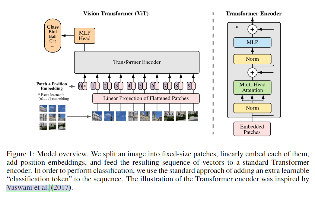
将图像分为了 $N$ 个 patch，每个 patch 的维度是 $P$，这样就可以将图像转换为一个序列，序列的长度是 $N$，维度是 $P$。需要单独再加一个 class token，用于表示图像的类别。

4. Incremental-DETR: Incremental Few-Shot Object Detection via Self-Supervised Learning

作者是新加坡国立大学和哈尔滨工业大学的学生

摘要

• Incremental 旨在学习新类别的目标检测，而不会影响到已有类别的目标检测。
• novel class 数据量少
• 通过在 DETR 上进行 fine-tune 和 self-supervised learning 来实现。
• 用到了 selective search algorithm
• 用到了 knowledge distillation
• code

引言

• 增量学习一直都是一个难题，很容易出现 catastrophic forgetting。
• 前人通过同时训练 base class 和 novel class 来解决，但是如果我们没有 base class 的数据，方法就会受限。
• 前人在 Faster R-CNN 做过类似的事情，第一阶段在 base class 上训练，第二阶段冻结类无关提取器和 RPN，只对预测头进行 fine-tune。作者深受启发。
• 作者解冻不同的DETR层进行微调，并根据经验确定投影层和分类头是特定于类的，DETR的CNN主干、变压器和回归头与类无关
• 假定在进行 incremental 的时候，base class 的数据是不可用的。
• 第一阶段：base model 预训练，之后进行 self-supervised fine-tune。第二阶段：在 novel class 上进行 incremental fine-tune。
• 第一阶段用到了 slecetive search algorithm
• 提出了 classification distillation loss 和 masked feature distillation loss
• dataset：COCO、PASCAL VOC

相关工作

• Object Detection
• Few-Shot Object Detection
• Incrementa Few-Shot Object Detection

问题定义

• $D_{novel}$ 用的时候 $D_{base}$ 不可用
• 新类和旧类没有重叠
• 新类仅有少量样本

方法

Base Model Training

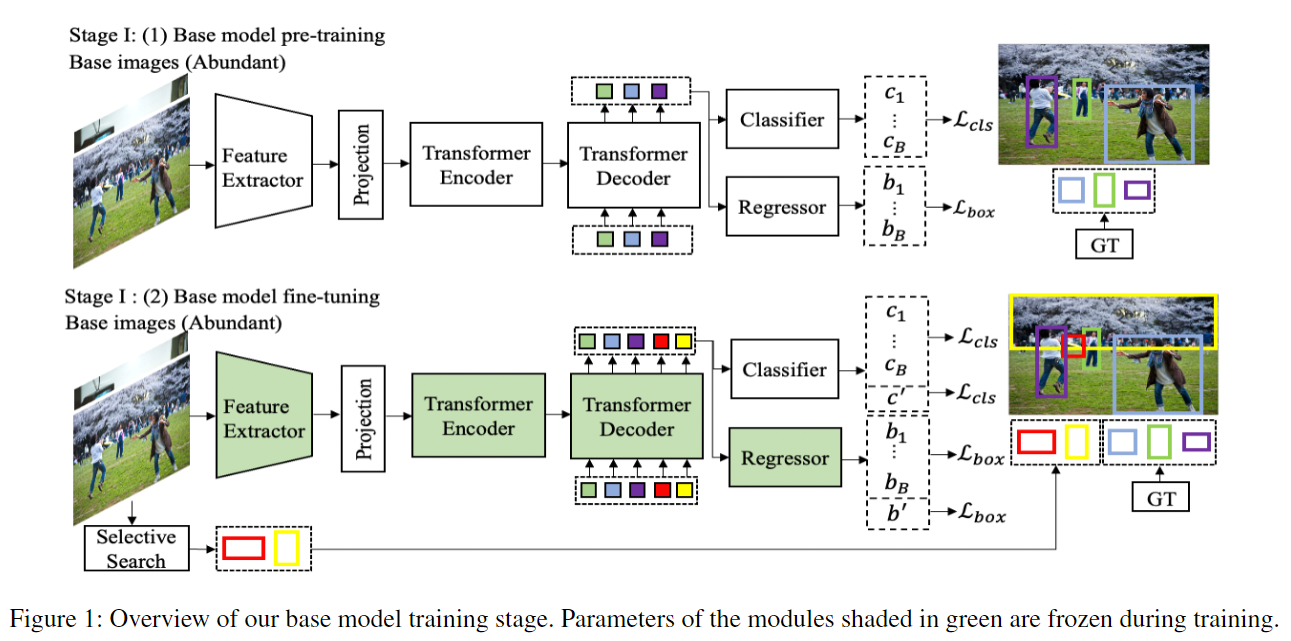
1. 在 stage 1 的第一部分，采用正常的 DETR 训练策略在 $D_{base}$ 上进行训练。
2. 在 stage 1 的第二部分，进来一张图片，通过 selective search algorithm 生成一些 proposals，之后选择 top O 个 proposals，要求这些 proposals 与 base class 的 ground truth bounding box 不重叠。之后将这些 proposals 作为 pseudo ground truth，采用 DETR 的方式进行训练。也就是图中的 $b'$，对应的类别是 $c'$。

• 找框：

$\hat{\sigma} = \text{arg} \quad \text{min}_{\sigma \in \mathcal{\sigma}\_N} \sum_{i=1}^N \mathcal{L}_{\text{match} }(y_i, \hat{y}_{\sigma(i)})$ $\mathcal{L}_{\text{match} }(y_i, \hat{y}_{\sigma(i)}) = - \mathbb{1}_{\{c_i \neq \emptyset\} } \hat{p}_{\sigma(i)}(c*i) + \mathbb{1}*{\{c*i = \emptyset\} } \mathcal{L}*{\text{box} }(b*i, \hat{b}*{\sigma(i)})$

• Hungarian loss：

$L*{hg}(y, \hat{y}) = \sum*{i=1}^N [- \log \hat{p}_{\hat \sigma(i)}(c_i) + \mathbb{1}_{\{c_i \neq \emptyset\} } \mathcal{L}_{\text{box} }(b_i, \hat{b}_{\hat \sigma(i)})]$

• 在 stage 1 中的第二部分，损失为：

$\mathcal{L}^{base}_{total} = \mathcal{L}_{hg}(y, \hat{y}) + \lambda' \mathcal{L}\_{hg}(y', \hat{y}')$

Incremental Few-Shot Fine-Tuning

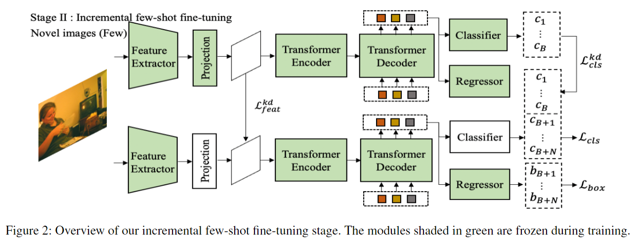
• 仅白色部分进行 fine-tune
• 直接 fine-tune，会导致 catastrophic forgetting，因此作者提出了 knowledge distillation。直接 knowledge distillation 会和 novel class 的学习产生冲突，所以这里引入了 $\mathcal{mask}^{novel}$，（如果是 novel class ground truth boxes，则为 1，否则为 0）。具体而言：

$\mathcal{L}^{kd}_{feat} = \frac{1}{2 N^{novel}} \sum_{i=1}^{w} \sum*{j=1}^{h} \sum*{k=1}^{c} (1 - \mathcal{mask}^{novel}_{ij}) ||f_{ijk}^{novel} - f*{ijk}^{base}||^2$ 其中，$N^{novel} = \sum*{i=1}^{w} \sum*{j=1}^{h} (1 - \mathcal{mask}^{novel}*{ij})$，$f^{base}$ 和 $f^{novel}$ 分别是 base model 和 novel model 的 feature map。$w$，$h$，$c$ 分别是 feature map 的宽、高和通道数。

直观理解，对于每一个像素点，对于它的所有通道，去看它是否是 novel class bounding box 的一部分，如果是，则不需要进行 knowledge distillation，否则，则需要进行 knowledge distillation。

同样，对于分类器头，直接做 knowledge distillation 也不合适，为解决这个问题，如下：

$\mathcal{L}^{kd}_{cls} = \mathcal{L}_{\text{kl\_div}}(\log(q^{novel}), q^{base})$

进来一张 novel image，通过 base model 进行预测，如果 class probability 大于 0.5，且 bounding box 与 novel class ground truth boxes 不重叠，则认为需要蒸馏，算 KL 散度。

• stage 2 的损失为：

$\mathcal{L}^{novel}_{total} = \mathcal{L}_{hg}(y, \hat{y}) + \lambda*{feat} \mathcal{L}^{kd}*{feat} + \lambda*{cls} \mathcal{L}^{kd}*{cls}$

实验

结论

• 通过蒸馏学习，做到了在学习新知识的同时不遗忘旧知识。
• 提前通过 self-supervised 生成一些 新类标签，进行fine-tune，使得模型更容易接受新知识。
• 断定模型中的部分可以分为 class-specific 和 class-agnostic 两部分。

5. Lightweight Transformer for Multi-Modal Object Detection (Student Abstract)

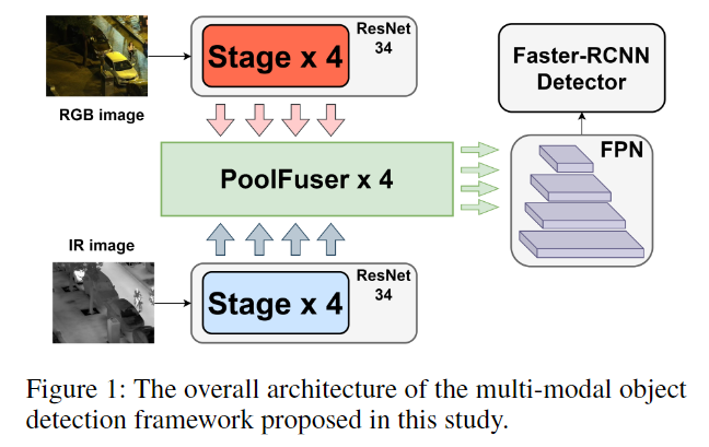
模型训练时，可以从多个角度进行训练，角度越多越准确，但却更慢。

比如自动驾驶，仅有一个传感器肯定没有多个传感器的结果准确，但是多个传感器的结果又太慢。

那么能不能又快又准呢？那就要从模态融合入手。作者提出了一种新的融合操作符，叫做 Poolformer-based fusion operator。

本质上来讲，本文更换了权重分配的方式，用 pooling 来进行替代，这样可以减少参数量，提高速度，但效果却不差。文章没有提供代码，但是作者回复邮件推荐了一份代码

6. Self-supervised Label Augmentation via Input Transformations

一言以蔽之，通过数据增强的方式来增强原始标签，不仅仅对于无监督、半监督学习有效，对于全监督学习也能带来效果的提升。将共享底层特征改成了 unified task

共享底层特征：先前的工作通常为原始任务和自监督任务维护两个独立的分类器（但共享公共特征表示），并同时优化它们的目标。也就是，不论你图像怎么变（增强），特征表示不能变。

• code

有效地利用基于 transformation 的自我监督进行全监督的分类任务。对于 few-shot and imbalanced classification scenarios 也有效果

Difference with previous approaches:

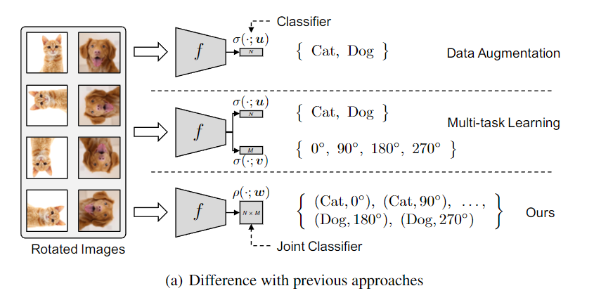
• 单纯的 Data Augmentation，只是对输入进行了变换，但却强行使得标签不变的一种方案，这种方案有一定弊端，比如：6 和 9，详见原文

$\mathcal{L}_{DA}(x,y;\theta,\mu) = \frac{1}{M} \sum_{j=1}^M \mathcal{L}\_{CE}(\theta(\hat{z_j}; \mu), y)$

• Multi-task Learning 同时学习两个任务，同时优化它们。但是，当数据集是全标签时，这种方法通常不会带来效果的提升。

$\mathcal{L}_{MT}(x,y;\theta,u,v) = \frac{1}{M} \sum_{j=1}^{M} \mathcal{L}_{CE}(\theta(\hat{z_j};\mu), y) + \mathcal{L}_{CE}(\theta(\hat{z_j};v),j)$

• 本文所提出的SLA(Self-supervised Label Augmentation)方法直接学习联合概率分布。效果最好，也最通用。

$\mathcal{L}_{SLA}(x,y;\theta,\omega) = \frac{1}{M} \sum_{j=1}^{M} \mathcal{L}\_{CE}(p(\hat{z_j};\omega), (y,j))$

此处损失详见原文。

对比效果如下：

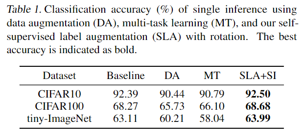
SLA 仅增加了标签的数量，对于模型的参数基本上没有影响。 SLA 可以弱化为 Data Augmentation，也可以弱化为 Multi-task Learning。但是 Multi-task Learning 约束太强（强制 label 不变），难以优化。

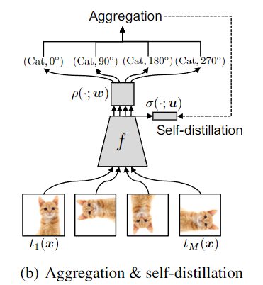
由于预测的结果变为了以前的 M 倍，所以先做 Aggregation，也就是把对应的 M 个条件概率加起来，然后再进行 softmax。之后和原来的标签进行交叉熵计算蒸馏损失。

$\mathcal{L}_{SLA}(x,y;\theta,\omega,\mu) = \mathcal{L}_{SLA}(x,y; \theta, \omega) + \mathcal{D}_{KL}(P_{aggregated}(·|x)|| \sigma(z;\mu)) + \beta \mathcal{L}\_{CE}(\sigma(z;\mu), y)$

7. Learn More for Food Recognition via Progressive Self-Distillation

• 面临的问题：

食品识别一直是一个比较困难的任务，因为这是一个比较细粒度的任务。例如对于鸟的识别，找到鸟头、爪子就好了，但是食品可能是各种水果、蔬菜堆叠在一起构成沙拉，这比较困难。传统的方法是先用弱监督的方式做很多位置的定位，之后聚合并抽取特征，最后分类。但这样一来，性能就会被位置定位所限制。我们很难把每一部分区域都学好。

• 解决方案：

作者提出了 PSD（Progressive Self-Distillation），用于去挖掘图像中更有用的区域。teacher model 和 student model 共享相同的 embeding。最后 inference 阶段，仅保留 teacher model。仍然属于 self-supervised 的范畴。

embedding 可以用 CNN，也可以用 transformer(e.g.,Swin Transformer)。

• dataset：ETHZ Food-101、Vireo Food-172、ISIA Food-500
• code: 无

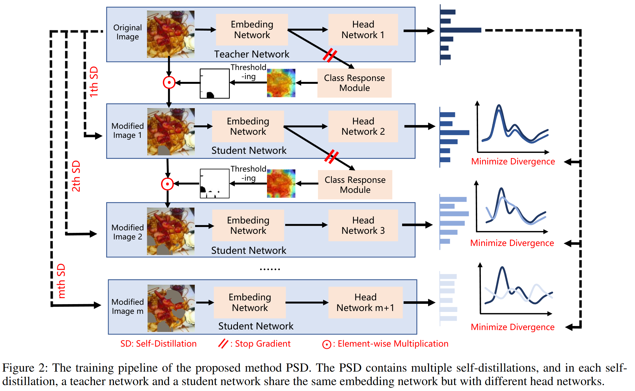
student model 和 teacher model 共享同一个 Embeding Network，但是有不同的分类器。输入原始图片给 teacher model，经过一个 ViT 得到一个 T x D 的 tokens，reshape 成 H x W x D 的 feature map，之后经过全局平均池化，得到一个 D 维的向量，之后经过一个全连接层，得到一个 C 维的向量，之后送入 Class Response Module。根据 Threshold，得到一个 mask，之后将 mask 与原始图片相乘，得到一个新的图片，送入 student model。如法炮制，进得到了很多的 student model。蒸馏阶段，使用 teacher model 的输出作为 ground truth，student model 的输出作为预测值，计算 KL 散度。

损失如下：

$\mathcal{L} = \mathcal{L}_{g}(x,y) + \sum_{i=1}^{m}(\omega*l \mathcal{L}*{l}(\hat{x}_{i-1}, y) + \omega_d \mathcal{L}_{d}(x, \hat{x}_{i}))$ 其中 $\mathcal{L}_{g}(x,y)$ 是原始的分类损失，$\mathcal{L}_{l}$ 是 locating loss，$\mathcal{L}_{d}$ 是 distillation loss。 $\mathcal{L}_{g}(x,y) = \mathcal{L}_{CE}(h(f(x;\theta); \phi*t), y)$ $L*{l}(x,y) = \mathcal{L}_{ce}(GAP(f(x;\theta); \Theta), y)$ $\mathcal{L}\_d(x, \hat{x}) = \mathcal{D}_{KL}(h(f(x;\theta); \phi_t), h(f(\hat{x};\theta); \phi_s))$

所谓渐进，是依靠$\omega_l$ 和 $\omega_d$ 来控制的。

$\omega_d = \begin{cases} \alpha \cdot \exp(-5(1 - \frac{e}{\beta})^2), & e < \beta \\ \alpha, & e \geq \beta \end{cases}$

垃圾文章，没有代码，作者邮件不回。$L_l$也没有讲清楚。Class Response Module 出来之后怎么进行 Threshold？怎么得到 mask？这些都没有讲清楚。或许需要一些食物识别的先验知识。

8. Solving Math Word Problems concerning Systems of Equations with GPT-3

摘要

本文解决了一个专业领域的问题，就是数学方程式的提取和求解问题。作者将其归到了 NLP 的范畴，使用了 GPT-3 来解决这个问题。 问题分三步：

1. 对问题进行 分类，是几元方程式。这个问题目前 GPT-3 能够达到 80%-100% 的准确率。
2. 提取方程式，这个问题的精度随着给定模型的例子数量的增加而增加。one-shot 的精度为 31%，3-shot 的精度为 69%。之后再进一步进行 fine-tune，精度可以达到 80%。
3. 生成新的问题，GPT-3 的精度在 33%-93%，具体取决于问题类型。

引言

本文聚焦的问题是 二元一次线性方程组，也就是两个变量，两个方程式。如上所述，解决问题如下：

• Q1: How good is GPT-3 at classifying problems into different themes?

• Q2: How good is GPT-3 at extracting a system of linear equations directly from problem descriptions?

• Q3: How good is GPT-3 at creatively generating valid problems?

• dataset

如下为 Q1. Table1: Instance problem from each category

类别

问题

Sum and Difference (S&D)

The sum of half of a number, x, and another number, y, is -28. The difference of x and y is 7. Find x and y.

Item and Property (I&P)

Three apples and four bananas cost $4.85. Three apples and ten bananas cost$8.75. Find the cost of an apple.

Perimeter of Rectangle (PoR)

The length of a rectangle is 3 cm less than double the width, and the perimeter is 53 cm. Find its dimensions.

Motion (MO)

Joey and Natasha start from the same point and walk in opposite directions. Joey walks 4 km/h faster than Natasha. After 2 hours, they are 31 kilometers apart. How fast did each walk?

Mixture (MI)

Twelve gallons of a 31% acid mixture is obtained by mixing a 23% solution with a 48% solution. How much of each must be used?

生成表达式的时候，前缀、中缀和后缀的进度不同。

已经有人通过 Transformer 来解决这个问题，但是作者说泛化性不好。详见文章的 Prior Applications of Transformers to MWP。还有人通过 BERT 来解决这个问题。

目前关注的问题是以下五个，作者仅考虑了其中的三个：

• identify the type of problem
• output step-by-step instructions
• extract the correct system of linear equations
• successfully solve the equations
• generate similar problems for users to practice.

Table 2: Extraction task example.

Problem

How many gallons of a 20% antifreeze solution and a 10% antifreeze solution must be mixed to obtain 40 gallons of a 16% antifreeze solution?

Valid Response

0.2x+0.1y=0.16*(x+y);x+y=40

Invalid Response

20x+10y=16*40 (only one equation is derived)

Invalid Response

20x+10(40-x)=16(40) (failed to use required variable y)

Invalid Response

2x+1y=40;0.2x+0.1y=0.16 (incorrect interpretation)

Table 3: Problem generation.

problem given in prompt

The larger of two numbers is 10 more than twice the smaller. If the smaller is subtracted from the larger, the result is 26. Find the numbers.

within-topic generation outcome

The larger of two numbers is 15 more than twice the smaller. If the smaller is subtracted from the larger, the result is 33. Find the numbers.

cross-topic generation outcome

The larger of two angles is 10 more than twice the smaller. If the smaller is subtracted from the larger, the result is 26. Find the angles.

9. Curriculum Temperature for Knowledge Distillation

• code

• Project Page

• 中文解读

• 引言中指出：MKD (Liu et al. 2022) 比较重视 数据增强。

• 相关工作中指出：

  • This training strategy has been widely applied in various domains, such as computer vision (Wu et al. 2018; Sinha, Garg, and Larochelle 2020) and natural language processing (Platanios et al. 2019; Tay et al. 2019).
  • Curriculum Dropout (Morerio et al. 2017)

10. Sharpness-Aware Minimization for Efficiently Improving Generalization

• code
• Third-party library

cifar100 的结果：Percentage correct 96.08，最强结果。

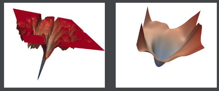
作者认为：现在模型的参数都特别多，单单靠 loss function 去做优化，不足以支撑起整个任务，这会导致太多不同的解。因此，作者提出了 SAM（Sharpness-Aware Minimization），通过优化 sharpness 来提高泛化性能，也就是优化曲率。

一言以蔽之：不仅仅要优化模型的 loss，还要优化 loss 最小值附近的 平滑度。可以将其视为一种学习算法，经测试，相当多的模型和任务，套用上这个算法，效果都会有所提升。

Theorem (stated informally) 1. For any $\rho$ > 0, with high probability over training set $S$ generated from distribution $\mathcal{D}$,

$\mathcal{D}(\omega) \leq \text{max}_{|| \epsilon ||\_2 \leq \rho} \mathcal{L}_{S}(\omega + \epsilon) + \mathcal{h}(|| \omega ||\_2^2 / \rho^2)$

where $h : R_+ → R_+$ is a strictly increasing function (under some technical conditions on $L_D (w)$).

事实上，上述公式的右侧可以写为：

$[\text{max}_{|| \epsilon ||_2 \leq \rho} \mathcal{L}_{S}(\omega + \epsilon) - \mathcal{L}_{S}(\omega)] + \mathcal{L}\_{S}(\omega) + \mathcal{h}(|| \omega ||\_2^2 / \rho^2)$

其中最后一项可以看成是一个正则项，可以用$\lambda || \omega ||_2^2$来代替。[]内的代表锐度，也就是 sharpness。中间那一项是 loss。

故而，SAM 的损失函数为：

$\text{min}_{\omega} \mathcal{L}_{S}^{SAM}(\omega) + \lambda || \omega ||_2^2 \quad \text{where} \quad \mathcal{L}_{S}^{SAM}(\omega) \stackrel{\triangle}{=} \text{max}_{|| \epsilon ||\_p \leq \rho} \mathcal{L}_{S}(\omega + \epsilon)$

就是一个最大最小化问题，详细推导见原文。

Because SAM’s performance is amplified by not syncing the perturbations, data parallelism is highly recommended to leverage SAM’s full potential (see Section 4 for more details).就是数据并行，效果更好。

11. Adaptive Hierarchy-Branch Fusion for Online Knowledge Distillation

13. Class Incremental Learning for Task-Oriented Dialogue System with Contrastive Distillation on Internal Representations (Student Abstract)

本文通过对比、蒸馏等技术来实现增量学习，用于对话系统。

通过以下几种方式来保证增量学习的效果：

• 仅更新部分相关新任务的参数
• 对比学习：新任务中的数据作为 anchors，原数据作为负样本。上一阶段模型和新阶段模型对于新任务数据的输出作为正样本对。简而言之，学习新任务的时候，不仅仅学习新任务的知识，还要学习新任务和原任务的区别。
• 复杂的损失函数：包括对比损失、交叉熵损失、蒸馏损失等。相互协调，妄想达到最好的效果。
• 动量更新：保证模型的稳定性。

作者并未提供代码，也无邮件回复。一言以蔽之，将各种东西混合在一起构成一套灌水垃圾。

14. Improving Training and Inference of Face Recognition Models via Random Temperature Scaling

本文针对人脸识别，介绍了不确定的问题。

模型对于无效的输入，仍然会以高置信度做出预测，这是不合理的。对于人脸识别，同样的人但是不同的照片，应该被映射到同一个 latent space，但这很难做到。

作者提出了 RTS（Random Temperature Scaling），将温度与不确定性相关联，通过随机温度缩放来影响模型的不确定性。

上述皆为论文中内容，实际上，如文中 Eqn.4 和 Eqn.5 以及 Fig.2 所示，作者提出了一种新的损失函数（类似softmax）,并引入了 Gumbel 分布。详见原文。

无代码，垃圾文章。

15. De-biased Teacher: Rethinking IoU Matching for Semi-supervised Object Detection

假code

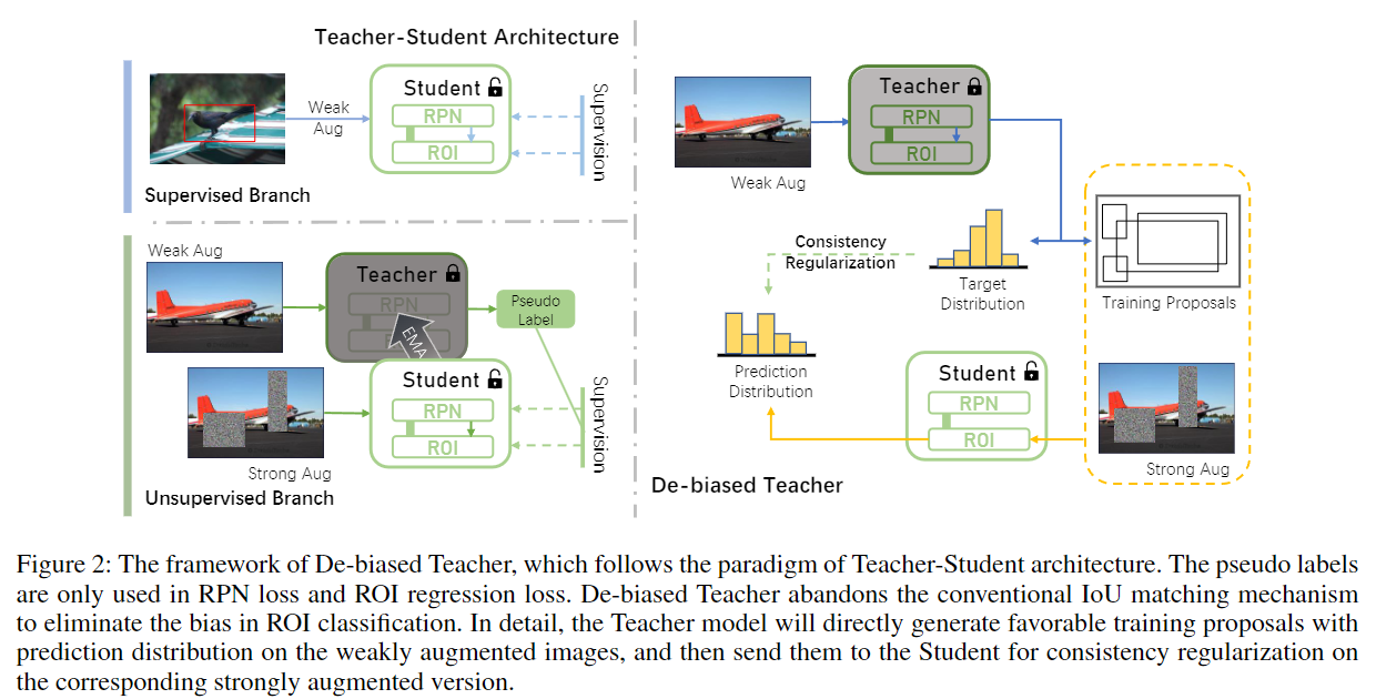
• 从 $D_{labeled}$ 和 $D_{unlabeled}$ 中采样 input。

  • labeled images 直接通过 weakly augmented 来训练 student model。
  • unlabeled images，Teacher 通过 weakly augmented 来生成 pseudo labels，之后通过 strong augmented 来训练 student model。作者称之为 一致性正则化。

• student model 通过 loss 进行训练更新，teacher model 通过自身和 student model 进行动量更新，详见 Eqn.1。

也就是说，本文三个贡献：

1. 一致性正则，和蒸馏的区别在于，teacher 和 student 都动。
2. teacher 通过 student 来进行动量更新。
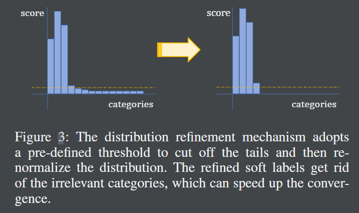
3. 截断 softmax 的尾部，阈值为 0.05。（推测没有使用温度系数T）

什么时候阶段？如何阶段？TODO

16. Grouped Knowledge Distillation for Deep Face Recognition

无 code. 已发邮件，未回。

$L = \mathcal{L}_{cls} + \mathcal{L}_{kd}$

其中 $\mathcal{L}_{cls}$ 是一个专门针对于人脸识别的损失函数。

一言以蔽之，作者将 logit 按照阈值进行分组。分别是 Primary-KD, Secondary-KD, and Binary-KD。**Primary-KD 用于学习主要的知识，Secondary-KD 用于学习次要的知识，Binary-KD 用于确保教师和学生之间的知识分布的一致性。**作者表示，Primary-KD 和 Binary-KD 是重要的，Secondary-KD 是累赘。

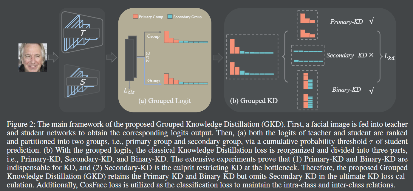
Binary-KD 参见原文公式 6，实际上就是一个二分类问题，用于确定分类是 Primary-KD 还是 Secondary-KD。

**注意 Fig.2 中的文字描述，作者指出根据 student 的输出进行 rank，之后开始累加，直到累加的值达到了 阈值，这部分就是 Primary-KD。teacher也排序。**此处有两个问题：

1. 这样排序，岂不是会出现类别不匹配的问题？
2. 根据 student 进行 rank 有什么用？不是应该根据 teacher？

作者还在 Method 文字的上面指出 feature distillation 优于 logit distillation。不敢苟同。

作者测试最好的阈值为 0.93，但作者的理论是错误的，所以也并无太多参考价值。

作者 Equ.3 的绝对值加的很好，值得借鉴，根据 teacher 进行排序的话，应该确实是可行的，可以做到自适应调整 Primary-KD 和 Secondary-KD 的比例，但要想做到类型匹配，需要存原来的索引，这样会造成计算成本的增加。

作者最后做了一个 masked face recognition 的实验，这手操作值得学习。

作者已回邮件，rank 时对 index 重新组织，并且代码中是根据 teacher 进行 rank. 但匪夷所思的是，作者说最后通过 student 进行 rank 反而会取得更好的结果。